- SPEECH
The 2021-2022 inflation surges and the monetary policy response through the lens of macroeconomic models
Speech by Philip R. Lane, Member of the Executive Board of the ECB, at the SUERF Marjolin Lecture hosted by the Banca d’Italia
Rome, 18 November 2024
Introduction
My aim today is to explain how macroeconomic models can help in understanding the extraordinary 2021-2022 inflation surges and the monetary policy response, in the context of the euro area.[1] By and large, the scale and persistence of the inflation surge surprised the central banking community, external experts and market participants. The unexpected nature of the inflation surge triggered many questions about the performance of macroeconomic forecasters.
At the same time, macroeconomic models can help us understand why the baseline projections did not foresee the inflation surge in its full scale and speed, while shedding light on the possible mechanisms and channels that may have been missed or under-stated. Scenario analysis has been enhanced and new models have been developed to enrich our understanding of the shocks that hit the economy over this period, as well as the mechanisms through which these shocks were transmitted to inflation. Models also play a central role in constructing some of the measures of underlying inflation that the Governing Council uses as an important cross-check for the inflation outlook. And models are essential in constructing policy counterfactuals to assess whether alternative monetary policy responses might have substantially reduced the scale of the inflation surge. Models therefore play an important role in strengthening our understanding of the recent inflationary surge and assessing the monetary policy response.
Model-based retrospective analysis provides several insights into the 2021-2022 inflation surges. The large forecast errors in the inflation outlook over this period were driven, at least initially, by energy and commodity price shocks, especially following the Russia-Ukraine war, and pandemic-related bottlenecks. Subsequently, changes in the transmission of shocks through the pricing chain, and in the behaviour of firms and consumers, likely played an important role in amplifying and propagating these shocks across the economy, converting relative price shocks into a general inflation shock.
Supply shocks, primarily originating from external sources, were key drivers of the inflation surges. While global and domestic surges in sectoral demand patterns also contributed to sectoral demand-supply mismatches (in the goods sector in 2020-2021 during the most intense phases of global pandemic lockdowns; in the services sector in 2022 during the post-pandemic reopening phase), the overall level of aggregate demand in the euro area was only barely above pre-pandemic levels by the end of 2022.
The pre-dominant role of supply shocks, combined with the fact that inflation expectations were initially signalling significant downside risks, supported the initial looking-through approach for monetary policy. In this context, it is also essential to recall the sequential nature of the shocks: the focus in 2021 was on pandemic-related supply disruptions and sectoral demand-supply mismatches, while the unjustified Russian invasion of Ukraine in February 2022 subsequently triggered extraordinary jumps in gas and oil prices.[2] The post-pandemic full-scale reopening of contact-intensive services sectors also took place in early 2022, after the ending of Omicron-related lockdowns. Put together, the second and third quarters of 2022 saw an extraordinary cocktail of inflation shocks, between the war-related commodity and supply chain shocks and the demand-supply mismatches in the reopening contact-intensive service sectors.
If policymakers had had perfect foresight about the shocks that were about to hit the economy, interest rates would have been raised earlier and more sharply. However, conditional on the real-time information available to policymakers (including how this information shaped baseline macroeconomic projections), monetary policy decisions in 2021-2022 were broadly in line with the policy paths indicated by the macroeconomic models.[3] This assessment includes both the initial phase in which monetary policy did not respond to the early stages of the rise in inflation and the subsequent phase of a sharp and sustained tightening cycle. This monetary policy response was, and continues to be, an important contributor to the disinflation process. Macroeconomic models have played a central role in helping policymakers in charting this monetary policy course, through their roles in: (a) macroeconomic forecasting; (b) estimating underlying inflation; and (c) calibrating the appropriate interest rate path.
This assessment puts the spotlight on the quality of the information set available to policymakers, especially in relation to the macroeconomic projections. I will cover this topic in the next section.
The 2021-2022 inflation surges: what did models miss?
The inflation surges in 2021 and 2022 surprised professional forecasters, both at the ECB and across other institutions and countries.[4] Inflation turned out to be much higher and more persistent than had been projected. This is clear from the very large and persistent forecast errors at both short and medium-term horizons in the Eurosystem and ECB staff projections for headline and core inflation.
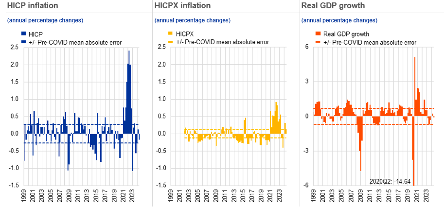
For example, forecast errors at the one-quarter ahead horizon during this period were more than five times larger than the average errors over the previous twenty years for headline inflation (and around twice as large for core inflation) and had the same direction for several successive quarters (Chart 1, left and middle panels). Indeed, the projection error in the December 2021 Broad Macroeconomic Projection Exercise (BMPE) for the year-over-year inflation rate at the end of 2022 was the largest ever, at around eight percentage points.
Projection errors were also materially larger than historical averages at medium-term horizons, with projections made early in the period suggesting that inflation would either return to target or fall below target well within the projection horizon. The errors in inflation at a four-quarter horizon, for example, were more than nine times larger during 2022 than the historic pre-pandemic average. This is important, since the medium-term inflation outlook is typically the most relevant for policymakers, given significant lags in the transmission of policy rate changes to inflation. The projection errors for GDP growth were smaller than for inflation, but still significantly above their historical range (Chart 1, right panel).
Chart 1
One-quarter-ahead errors in the inflation projections of Eurosystem/ECB staff
Sources: Eurosystem/ECB staff macroeconomic projections for the euro area and Eurostat.
Notes: An error is defined as the outturn for a given quarter minus the projection made for that quarter in the previous quarter (for example, the outturn for the fourth quarter of 2022 minus the figure projected for that quarter in the September 2022 ECB staff macroeconomic projections).
The latest observation is from the September 2024 ECB staff Macroeconomic Projection Exercise (MPE).
In understanding these large forecast errors over 2021-2022, it is important to differentiate between errors due to conditioning assumptions – especially linked to shocks to key variables such as energy or food prices – and errors in the way these assumptions were propagated through the forecasting models.
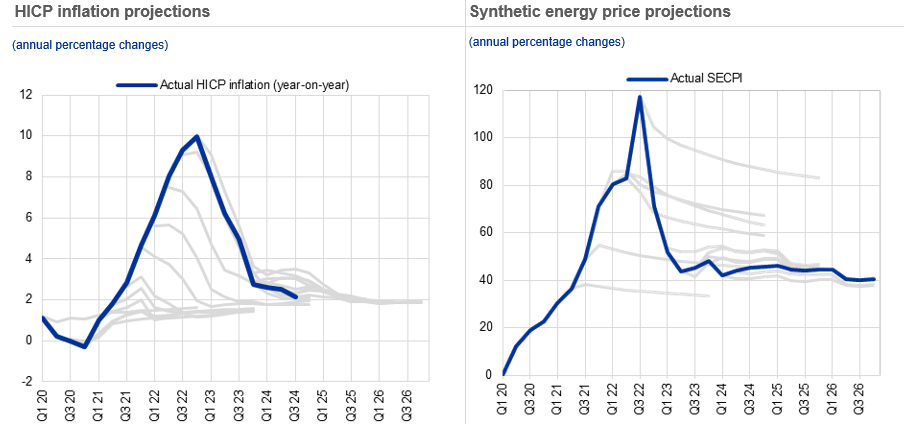
The starting point for the ECB staff projections is a set of conditioning assumptions for the future evolution of key input variables, known as “technical assumptions”.[5] For example, the paths for inputs such as commodity prices, including oil and gas prices, and short-term interest rates are based on market expectations at the time of the projection cut-off date.[6] The right panel of Chart 2 shows that the expected paths for oil and gas prices were revised up repeatedly over successive projection rounds at the end of 2021 and throughout 2022. This highlights how energy prices were repeatedly expected by markets – and therefore by our projection models – to decline. However, a sequence of upward surprises to energy prices materialised, especially following the Russian invasion of Ukraine. This sequence of shocks pushed up inflation and compounded forecast errors over successive projection rounds.
Chart 2
Headline inflation and energy composite projections from Q1 2020 to Q3 2024
Sources: Eurosystem/ECB staff projections and Eurostat for left-hand scale. Refinitiv and ECB staff calculations for right-hand scale.
Notes: Projections for the synthetic energy price index were introduced in 2021. Its methodology was changed in 2023. To account for this, projections before 2023 have been rebased to the new Synthetic Energy Commodity Price Index (SECPI) index.
The latest observation is from the September 2024 MPE for the left-hand scale and for the third quarter of 2024 for the right-hand scale.
In order to quantify the importance of energy price and other shocks in driving inflation projection errors, we can use models to construct counterfactual paths for inflation under a scenario in which forecasters had perfect foresight at each projection round about how energy prices and other conditioning variables would actually evolve over the projection horizon. This allows projection errors from incorrect technical assumptions to be isolated from the errors related to the transmission of shocks as embedded in models. Of course, the results from such a decomposition depend on the specific model. It is also important to keep in mind that the ECB/Eurosystem staff macroeconomic projections are not purely model based but also include staff judgement.[7]
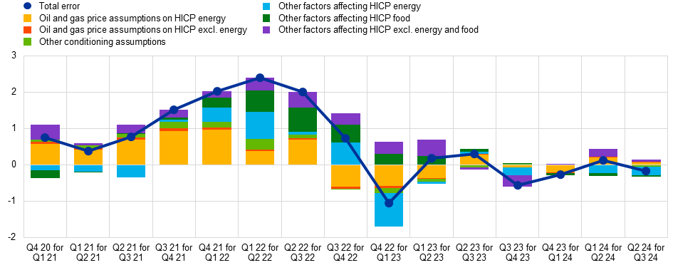
One way to carry out this counterfactual exercise is to use the Basic Model Elasticities (BMEs) of the Eurosystem national central banks (NCBs), which summarise the key relations between projection variables.[8] This exercise suggests that a substantial share of forecast errors for inflation during 2021 and 2022 was due to errors in the technical assumptions.[9] For example, errors in assumptions about oil and gas prices accounted for the majority of the one-quarter ahead inflation projection error until early 2022 (yellow and green bars in Chart 3).[10] Subsequently, however, the importance of other factors affecting food and core inflation grew in importance.
Chart 3
Decomposition of recent one-quarter-ahead HICP inflation errors in Eurosystem/ECB staff projections
(annual percentage points; percentage point contributions)
Source: ECB calculations.
Notes: “Total error” is the outturn minus the projection. The labels on the horizontal axis indicate the quarter in which the projections were published and the quarter to which those projections relate (i.e. “Q4 20 for Q1 21” denotes projections for the first quarter of 2021 that were published in the fourth quarter of 2020). The decomposition is based on updated elasticities derived from Eurosystem staff macroeconomic projection models as at late 2023. “Other assumptions” refers to exchange rates, short and long-term interest rates, stock prices, foreign demand, competitors’ export prices and food prices”.
The latest observation is from the June 2024 Eurosystem staff Broad Macroeconomic Projection Exercise (BMPE).
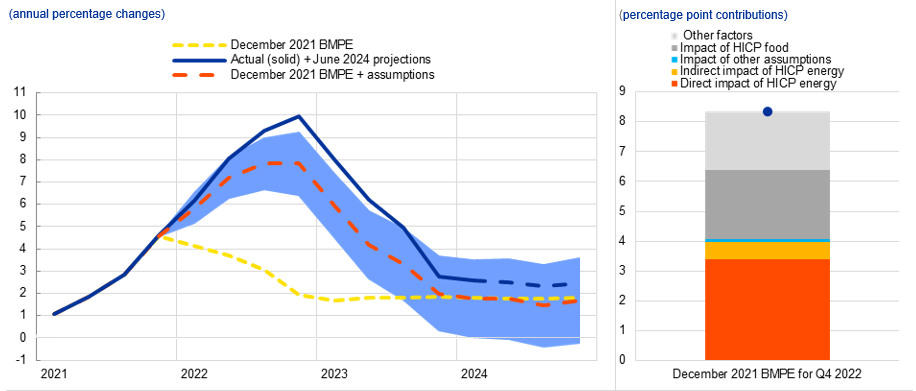
Further insight can be gained by running this counterfactual exercise in a fully-fledged macroeconomic model. ECB-BASE is the workhorse large-scale estimated semi-structural model used at the ECB to support and cross-check the staff projection exercises.[11] Decomposing the eight percentage point projection error at the peak of inflation in the fourth quarter of 2022 – relative to what had been projected in December 2021 – confirms that around half was due to unexpected developments in technical assumptions around oil and gas prices (red and yellow bars in Chart 4). Nearly one third, on the other hand, was due to errors in food inflation (dark grey bar in Chart 4), while the remainder was due to other factors that drove the error in core inflation (light grey bars in Chart 4). As such, errors in the set of technical assumptions go a long way towards explaining the forecast errors.[12]
At the same time, a sizeable share of the inflation forecast errors over this period cannot be explained by errors in the assumptions around energy and food prices. Two explanations for the remaining errors seem plausible.
The first explanation relates to statistical uncertainty. Macroeconomic forecasting models are underpinned by empirical estimates of model relations that are based on historical regularities. Statistical uncertainty around these estimates maps into statistical uncertainty around the central tendency of the inflation projection. Conditioning on the ex-post values for the technical assumptions, the statistical distribution around the inflation projections from the vantage point of December 2021 is relatively wide (Chart 4, blue area).[13] The actual inflation outturns (solid blue line in Chart 4) experienced during the inflation surge were close to the bounds of this model uncertainty, although inflation was still slightly too high to be compatible with the model in the second half of 2022 and the first half of 2023.
Overall, correcting for the actual path of energy prices and other conditioning variables, it cannot be ruled out that actual inflation was largely consistent with the historically-estimated statistical distribution around forecasts. This would imply that the economic relations estimated in the models to capture the transmission of shocks to inflation have remained broadly valid during the inflation surge, so long as the full statistical distribution is taken into account.
Chart 4
Decomposition of HICP inflation projection errors in December 2021 BMPE conditioning on December 2022 BMPE assumptions using ECB-BASE
Source: ECB-BASE, Eurostat, December 2021 BMPE and June 2024 BMPE.
Note: “December 2021 BMPE + assumptions” is simulated using the December BMPE baseline, but imposing the paths of HICP energy, HICP food and other technical assumptions from the June 2024 BMPE.
The second explanation is that economic relations might also have (temporarily) shifted during this extraordinary episode, including through an array of non-linear responses to the scale and combination of the shocks and the shift in the level of inflation. For example, in a high inflation environment, firms may adjust their prices more often than normal, in an attempt to pass on rapidly rising input and operational costs and protect their profits.[14] Furthermore, the broadening of the inflation shock from the energy sector (including via the food sector) to the services sector may also have been amplified during 2022 by the strong demand for contact-intensive services (tourism, hospitality) due to the reopening of these sectors after the final pandemic lockdowns. While costs were increasing quickly, the price elasticity of demand for services was plausibly atypically low due to this pandemic reopening phase, allowing for a greater pass-through of the cost shocks.
Furthermore, these conditions were ripe for a non-linear responses feedback loop between inflation and short-term inflation expectations. It is plausible that short-term inflation expectations are more sensitive to large inflation shocks than to small inflation shocks. Although longer-term inflation expectations remained broadly stable throughout, perceptions of past inflation and short-term expected inflation rates did increase in response to the inflation surges. In the event of a large inflation shock, an increase in near-term inflation expectations may take hold among households and firms, with firms anxious to avoid suffering relative price declines and households more likely to attribute individual price increases to general inflation than to a relative price increase.
Indeed, the evidence suggests that there was a marked increase in the frequency of price increases over the course of 2022 (Chart 5).[15] This state-dependent increase in the frequency of price adjustments resulted in the faster-than-normal pass-through of the unique and large sectoral shocks. In terms of the key Phillips Curve macroeconomic relation between slack and inflation (whether at aggregate or sectoral levels), this can be interpreted as some combination of a shift up in the curve and an increase in the slope of the Phillips Curve. And indeed, estimates from a time-varying parameter model show some increase in the slope of the Phillips curve from early 2021 (Chart 6, left panel). Furthermore, the evidence based on sectoral data also shows a shift in the correlation between sectoral capacity utilisation and sectoral prices increases (Chart 6, right panel).[16] While the 2021-2022 inflation surges should not be interpreted as primarily originating in the recovery of product and labour markets from the 2020 pandemic lows, the domestic rebound added to overall inflationary pressures. I return to the contribution of domestic demand in the next section.
Chart 5
Frequency of consumer price changes over time, by aggregate product category
(percentages)
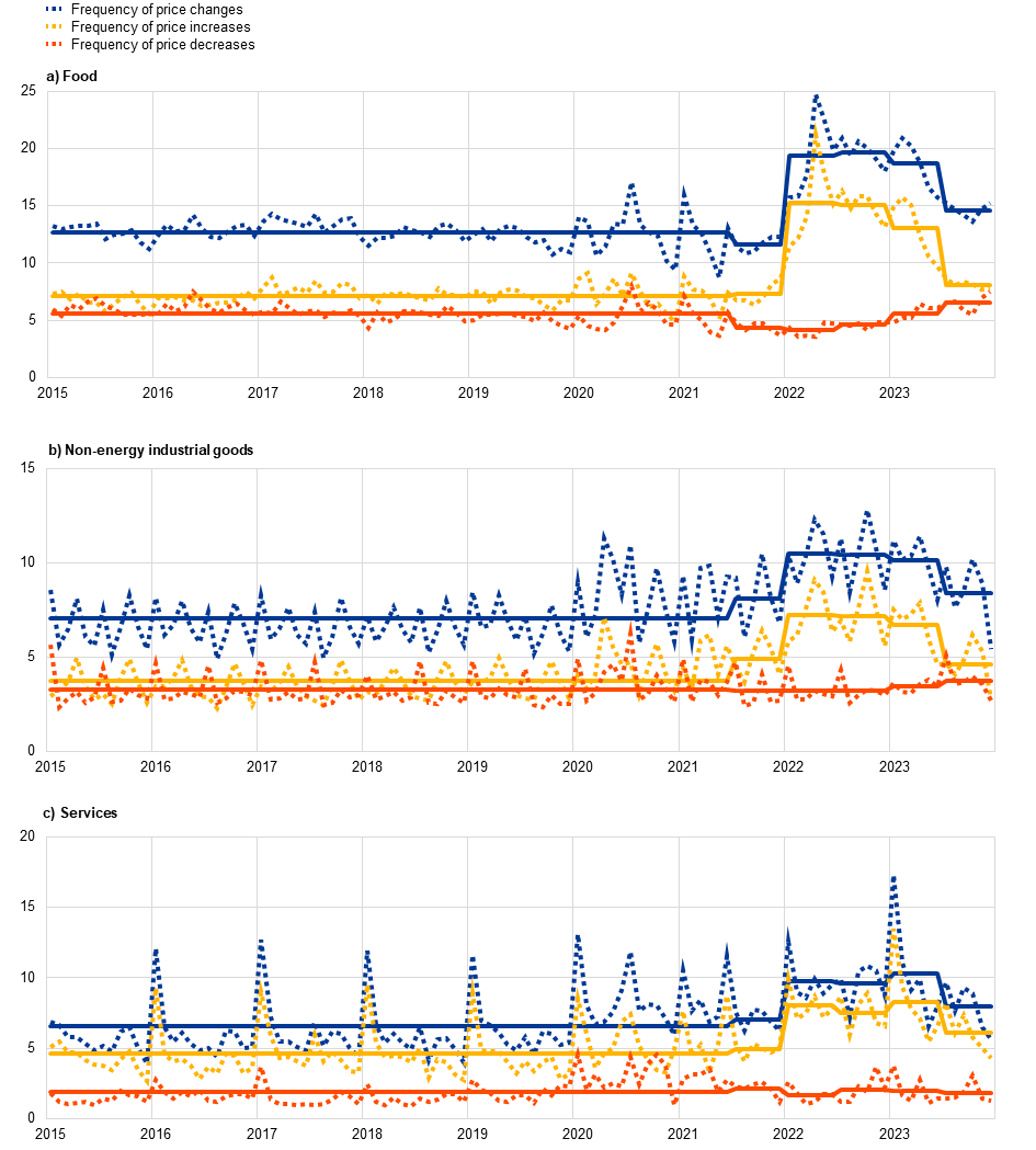
Sources: Consumer price micro-datasets from the national statistical institutes of Germany, Estonia, Spain, France, Italy, Latvia and Lithuania.
Notes: The chart shows the weighted average frequencies of price changes (excluding sales). VAT changes in Germany (2020-21) and Spain (2020-23) have been excluded. The solid lines plot the average over the period 2015-21 and half-year averages over the period 2021-23. The latest observations are for December 2023.
Chart 6
Increasing pass-through from slack to inflation
 |
|---|
Sources: Eurostat, DG-ECFIN and Eurosystem calculations.
Notes: Left chart: the Phillips curve specification relates the quarter-on-quarter growth rate of the seasonally adjusted HICP index to its own lag, capacity utilisation in industry, the lagged growth rate in import prices and medium-term survey-based inflation expectations. Time-varying parameter estimates where coefficients and log variance of residuals are assumed to follow a random walk. Right chart: services and manufacturing capacity utilisation are shown in deviation from the pre-COVID long-term average.
Faced with large forecast errors and significant uncertainty, ECB staff worked to develop new models and enhance the scenario analysis in the policy process. The new models developed include models of underlying inflation, satellite models that allow for alternative transmission channels, and machine learning models that try to allow for important non-linearities.[17] Each of these approaches can help to cross-check projections from the main forecasting models. In turn, the staff judgement element in the forecasting process enables the incorporation of the results from these supplementary analytical exercises, both in the baseline and in the risk assessment. No doubt the lessons learned from the 2021-2022 high inflation episode will prove to be especially valuable in the future if a similar configuration of shocks were to arise.
The recent experience certainly highlights the risks of over-reliance on baseline projections. Scenarios can be an effective way to represent risks when uncertainty is large or hard to quantify.[18] In 2020 and 2021, each set of quarterly staff projections included scenario analyses based on alternative assumptions regarding the future evolution of the pandemic and its economic consequences. In 2022, alternative scenarios focused on the economic consequences of the war in Ukraine, especially as regards uncertainties about energy supply. More recently, the scenario analysis has focused on more specific risks, such as a slowdown in the Chinese economy or a potential escalation of the conflict in the Red Sea area. In my May 2024 Stanford speech, I discussed how these alternative scenarios can be used to construct policy counterfactuals and will go into more details in a forthcoming speech on the use of scenarios to assess the robustness of alternative policy paths.[19] In addition to scenario analysis, the macroeconomic projections are accompanied by a large set of sensitivity analyses in relation to shifts in the technical assumptions and alternative parameter choices in model calibration.
Demand versus supply shocks
Models have also been deployed to interpret forecast errors through the lens of identified structural shocks and to quantify their contribution to inflation. Estimates from a large structural vector autoregressive (VAR) model – which employs sign and zero restrictions to identify the global and domestic demand and supply shocks driving deviations of inflation from the model-implied mean – indicate that external supply shocks were the main driver of the initial inflation surge in the euro area, although shocks to external demand and domestic demand also played a role, especially during 2022 (Chart 7).[20]
In particular, the shock decomposition points to various phases. The initial inflation increase was mainly driven by global supply shocks, related to supply chain disruptions, surging oil and gas prices and higher commodity prices more generally. These results supported an initially-circumspect monetary policy response, as the central bank still gathered evidence about the persistence of the inflation shock and its likelihood to affect materially expectations and other behavioural relations in the economy. In particular, in the absence of a clear understanding of the nature and expected persistence of the shocks, a more patient and deliberate policy response that weighs up the risks to different options, appeared appropriate.
In a second phase, the indirect effects from energy and food price spikes, as well as supply chain bottlenecks, passing through into core inflation led to the broadening of inflation pressures. Increasing demand, in particular in supply-constrained contact-intensive services, such as tourism and hospitality, added to inflationary pressures. Together with the risk that high inflation might de-stabilise inflation expectations, the increasing contribution of domestic demand add to the case for the aggressive monetary policy reaction that took place in this phase. In a third phase, as the energy and supply chain disruptions abated and monetary policy dampened demand, headline inflation started to decline rapidly.
Chart 7
Supply and demand drivers of inflation dynamics
(annual percentage changes and percentage change contributions; deviations from mean)
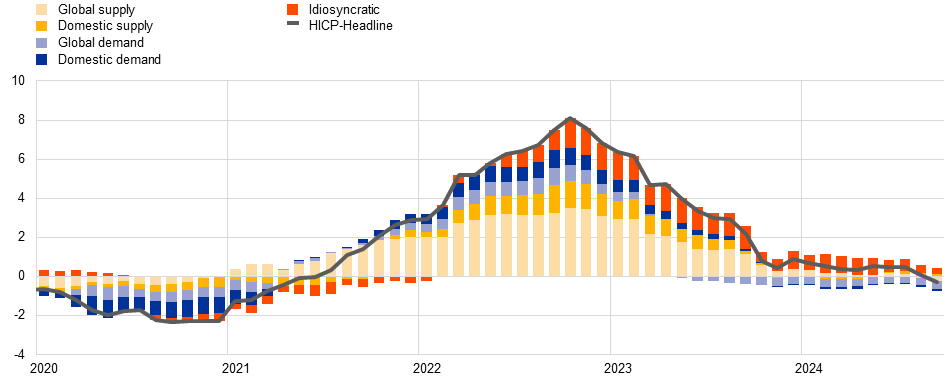
Sources: Eurostat, ECB, Eurosystem, and ECB staff calculations.
Notes: historical decomposition based on a large BVAR model accounting for a rich set of inflation drivers, identified with zero and sign restrictions, see Bańbura, M., Bobeica, E. and Martínez Hernández, C., (2024) “What drives core inflation? The role of supply shocks”, ECB Working Paper No. 2875. The chart shows the deviations of HICP inflation from the mean implied by the model.
The latest observation is for September 2024.
Of course, inference is sensitive to the type of model and the set of identifying assumptions.[21] A key challenge is to correctly capture the information set. A model needs to contain sufficient information to span the space of the structural shocks of interest. Otherwise, the correct shocks cannot be recovered from the history of observed variables. In stylised terms, the larger the model (or the more variables that are included), the more room there is to control for the different factors that affect inflation and, in particular, to separate out shocks from structural drivers.
This is particularly relevant when inflation is driven by a multifaceted and unusual set of shocks and structural drivers, originating both at home and abroad, as was the case over the 2021-2022 period. The dramatic fallout from the pandemic and the rapid bounce back following the reopening of economies after lockdowns are cases in point. In turn, amongst its many other effects, the shock of the Russian invasion of Ukraine constituted an extraordinarily-disruptive supply shock to the energy sector. As it turns out, models that rely on a small information set tend to assign a stronger role to demand factors and predict over-smooth dynamics of inflation and growth because such small-scale models are not designed to capture the type of sudden changes witnessed in that episode.[22]
The policy implications of model-based identification of demand and supply influences are not always easy to draw. That is, the policy implications not only depend on the source and nature of the shock but also its size and persistence. For example, a supply shock that is highly transitory (such as a temporary limitation in oil production in response to a short-lived geopolitical event) or a temporary surge in sectoral demand during the pandemic reopening phase (compounded by initially-limited supply capacity in the contact-intensive services sectors) may call for a looking-through policy response given the significant lags in the transmission of monetary policy.[23] By contrast, a string of large and persistent supply shocks in the same direction requires central banks to tighten in order to avoid longer-lasting inflation effects via wage-price spirals and dislocations in expectations.
In relation to the latter risk, the de-anchoring of longer-term inflation expectations warrants close monitoring, and models can help policymakers understand the risks of de-anchoring under alternative shocks and scenarios. For instance, simulations using a regime-switching DSGE model suggest that substantial downward de-anchoring risks prevailed throughout most of 2021, due to the low inflation of the previous periods exerting a persistent dampening effect on expectations as well as the initial inflationary shocks being largely understood to be temporary in nature.[24] The further increase in inflation in early 2022 saw a rapid decline in downward de-anchoring risks and an increase in upward de-anchoring risks. The forceful policy response over the course of 2022 and 2023 helped to limit, and then reduce, these upward de-anchoring risks (Chart 8). Later on, risks became more balanced as inflation came down tangibly.
Chart 8
Risks of de-anchoring of medium-term inflation expectations
(percentage risk of upside and downside de-anchoring risks)
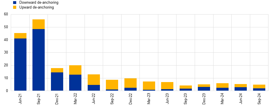
Sources: ECB calculations based on Christoffel, K. and Farkas, M. (2025), “Managing the Risks of Inflation Expectation De-anchoring”, IMF Working Paper Series, 2025, forthcoming.
Notes: The charts show the risk of de-anchoring for the staff projections from June 2021 to September 2024. The simulations are based on a regime switching version of the NAWM I (Christoffel, K., Coenen, G. and Warne, A. (2007)), where the credible regime is defined as the estimated version of the NAWM I, with a fixed inflation target, the de-anchored regime is characterised by a time varying inflation target. Upward de-anchoring is defined as a situation in a de-anchoring episode, where the perceived inflation target is above 2%. The share of de-anchoring is based on 1,000 simulations over a ten-quarter evaluation horizon.
The latest observations are from the September 2024 MPE.
The speed and strength of monetary policy transmission is also important when calibrating the appropriate monetary policy response.[25] Provided that monetary policy tightening transmits through to inflation in line with historical regularities, then our models should provide a good guide as to how fast and how far policy rates would need to be increased in response to the inflation shock. However, there is evidence that the aggressive rate hikes in response to inflation, and the highly restrictive monetary policy stance, have resulted in a faster-than-expected rise in lending rates as well as a larger contraction in credit flows, in particular to firms (Chart 9). This is important, because stronger-than-expected transmission would, all else being equal, call for smaller, or more gradual, rate increases in response to rising inflation.
Chart 9
Monetary policy transmission to firms and households compared to past cycles
(x-axis: years; y-axis: cumulative changes in percentage points for rates, credit growth in deviation from the start of the cycle (t) in p.p. for credit to firms and loans to households)
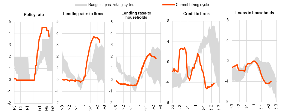
Sources: ECB (MIR) and ECB calculations.
Notes: The ECB relevant policy rate is the Lombard rate up to December 1998, the main refinancing operations rate up to May 2014 and the deposit facility rate thereafter. Starting months correspond to the month immediately preceding the first hike, or explicit announcement of the hike, of the cycle. The hiking cycles considered are those starting in June 1988, October 1999, November 2005 and May 2022. Credit to firms is the sum of bank loans and debt securities. Bank loans are adjusted for sales and securitisation and cash pooling. Lending rates refer only to bank loans.
The latest observations are for October 2024 for the policy rate and for September 2024 for lending rates, credit to firms and loans to households.
Cross-checking the outlook with measures of underlying inflation
The high level of uncertainty surrounding the inflation outlook over the 2021-2022 period called for the development of additional metrics to distinguish between temporary and more long-lasting inflation dynamics. Models played an important role in the development of underlying measures of inflation, which aim to filter out the short-term volatility in headline inflation and better capture the low-frequency component of inflation. Such metrics provide a useful cross-check to the inflation projections, especially in times of elevated uncertainty.
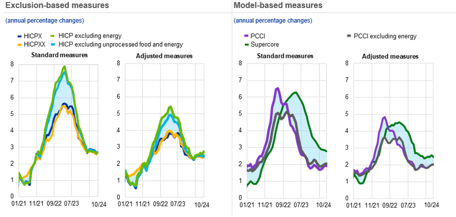
Most measures of underlying inflation have come down significantly from their peak (Chart 10).[26] Exclusion-based measures, which peaked around the beginning of 2023 have fallen steadily, and now sit just below three per cent. Model-based measures of Persistent and Common Component of Inflation (PCCI) measures, which have tended to perform the best in predicting HICP inflation since the pandemic, peaked earlier (around the middle of 2022) before declining quickly, and have now hovered around two per cent for several months.[27]
In interpreting measures of underlying inflation, it is important to keep in mind that these can be temporarily distorted by the economy-wide impact of cost shocks such as bottlenecks and energy shocks. Models can be used to “partial out” these influences from the underlying inflation measures to give a better sense of the medium-term dynamics of inflation. These adjusted measures had a significantly lower peak rate of underlying inflation than the unadjusted measures but, by construction, were also less affected by the sharp turnaround in energy prices and easing of supply bottlenecks during 2023 that flattered the speed of progress in the unadjusted measures.
Chart 10
Euro area underlying inflation measures and their adjusted counterpart
Sources: Eurostat and ECB staff calculations.
Notes: HICPX stands for HICP inflation excluding energy and food; HICPXX for HICP inflation excluding energy, food, travel-related items, clothing and footwear; PCCI is the persistent and common component of inflation, while Supercore aggregates HICPX items sensitive to domestic business cycle. See also Bańbura et al. (2023), “Underlying inflation measures: an analytical guide for the euro area”, Economic Bulletin, Issue 5, ECB. The “adjusted” measures abstract from energy and supply-bottlenecks shocks using a large SVAR, see Bańbura, M., Bobeica, E. and Martínez-Hernández, C. (2023), “What drives core inflation? The role of supply shocks”, Working Paper Series, No 2875, ECB, November.
The latest observation is for October 2024 (flash estimate) for HICPX, HICP excluding energy and HICP excluding unprocessed food and energy and September 2024 for the rest.
It is also important to understand what the various measures tell us about the speed and sequencing of the disinflation process. The delayed and lagged adjustment in indicators such as services inflation, domestic inflation and wage growth highlight that convergence to the medium-term target may still take time. It will be important to continue to monitor developments in domestic inflation, which has declined only slowly, mainly due to the delayed adjustment in services inflation, which itself is closely linked to wage developments.[28]
Policy counterfactuals
The complex shocks that hit the euro area economy in 2021 and 2022 and the high inflation which emerged also raise the question of the appropriate monetary policy response of the ECB. This can be analysed by constructing policy counterfactuals that give an indication of what would have happened to inflation had the ECB acted differently. Staff use macroeconomic models to build these counterfactuals in real time, under different assumptions for the policy rate path and the expected path for inflation and growth. But the same models can also be used to construct counterfactuals with the benefit of hindsight, thus providing insight on what appropriate monetary policy might have looked like had the extent of the inflation surge been known from the outset.
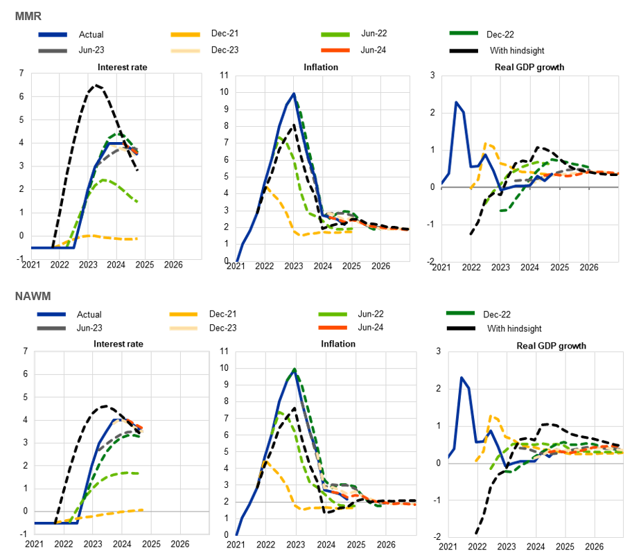
As an example, counterfactuals can be constructed using two policy models developed by ECB staff: the MMR model and the NAWM model.[29] Given projections for inflation and a measure of economic slack, as well as assumptions about the interest rate path, it is possible to construct policy paths that minimise a loss function featuring squared terms for the deviation of inflation from target, the output gap, and the change in the interest rate. The last term is a proxy for financial or other stress that could be created if the monetary stance changes very rapidly.[30] According to the model simulations, had the exact nature and size of shocks that were about to hit the economy been known back in the fourth quarter of 2021, the model-implied optimal policy (as defined by the minimisation of this loss function) would have called for interest rates to be increased earlier and more forcefully (Chart 11 black dashed). Inflation would have peaked at around 8 per cent rather than the 10 per cent observed in the fourth quarter of 2022. However, this tightening would have come with large output costs, with quarter-on-quarter growth rates 1 to 2 percentage points lower, depending on the model.
Of course, the ECB did not possess perfect foresight. The projections by ECB and Eurosystem staff, as well as those of other forecasters, predicted much lower and less persistent inflation as the baseline. In looking at the policy paths that were constructed using the actual information available to policymakers at the time – as reflected in the ECB/Eurosystem staff projections for inflation and growth – it shows the actual interest rate path during the hiking cycle was broadly in line with the model-implied optimal policy path (Chart 11, blue lines vs. coloured lines).
Chart 11
Optimal policy in real-time and with hindsight
(left panel: percentage per annum; middle panel: annual percentage changes; right panel: quarterly percentage changes)
Source: ECB calculations based on the MMR model (see Mazelis, F., Motto, R., Ristiniemi, A. (2023), op. cit.) with the exercises documented in the Handbook on Inflation (Coenen, Mazelis, Motto, Ristiniemi, Smets, Warne, Wouters (forthcoming)), and the NAWM II model (see Darracq Paries, M. Kornprobst, A., Priftis, R. (2024), op. cit.).
Notes: The optimal policy rate path simulations beyond the third quarter of 2024 are not shown for confidentiality reasons. “Actual” denotes historical data. The other dashed lines on the left graph are a sequence of optimal policy counterfactuals computed in real time at each projection vintage from the fourth quarter of 2021 to the second quarter of 2024. The “With hindsight” lines denote the optimal policy counterfactual computed in the fourth quarter of 2021 with the benefit of hindsight by assuming that the same information that we now have on subsequent inflation and output developments was already available in the fourth quarter of 2021. The middle and right panels show implied inflation and output growth respectively.
Chart 12
Early tightening counterfactual

Source: ECB calculations based on the MMR model (see Mazelis, F., Motto, R., Ristiniemi, A. (2023), op. cit.) with the exercises documented in the Handbook on Inflation (Coenen, Mazelis, Motto, Ristiniemi, Smets, Warne, Wouters (forthcoming)).
Notes: “Baseline” denotes historical data available in the third quarter of 2024. The solid lines in the left-hand side chart are the counterfactuals in Q4 2021 and Q2 2022 from Chart 11. Each of the lines with a marker on the left panel is a counterfactual rate path computed by constraining the lift-date to match the actual one and letting policy evolve optimally afterwards. The lines on the right panel are the difference in impact on inflation between the unconstrained and constrained case.
Two instances can be identified in the MMR model in which the model-implied optimal policy prescriptions differed slightly from the path of interest rates followed by the ECB. The first instance was in early 2022, when optimal policy would have called for interest rate hikes already in the first quarter. The implications of this delayed start to rate hikes can be assessed by comparing inflation outcomes under a counterfactual in which the optimal interest rate path is constrained not to increase until the time in which the ECB started increasing rates and under the alternative assumption that the rate path is unconstrained. The inflation outcomes in the two cases are very close to each other, in the order a few basis points, suggesting that small changes in the exact timing of lift off were not consequential: what matters in the model is the overall direction of travel of monetary policy rather than whether one rate action is brought forward or backward by one quarter. The second episode (not shown in the chart) was in September 2023 when the model-implied optimal policy would have called for one fewer interest rate hike.
However, the model-implied optimal policy path should be checked against an array of risk considerations. The optimal policy paths above are drawn around the central tendency of the BMPE projections: especially during periods of high uncertainty about the macroeconomic outcomes, it is prudent to also consider alternative scenarios. In particular, choosing a policy path that avoids the worst scenario from happening is a form of insurance and can in practice call for either a more aggressive or more gradual policy response than indicated by a simple loss function that is conditioned on the baseline projections.[31][32]
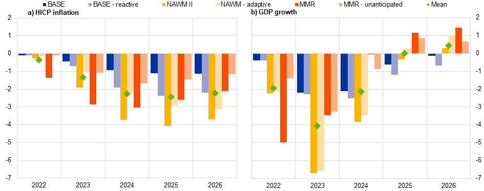
Policy models can also be employed to compute counterfactuals to quantify the impact of the actual monetary policy tightening on the disinflation process. The exercise is conducted using the ECB’s main policy models – NAWM, MMR and ECB-BASE.[33] According to these models, without the unprecedented tightening, inflation would have been about two percentage points higher on average in each year between 2023 and 2026 (Chart 13). The exact effects of monetary policy on inflation and output are subject to significant uncertainty and depend, among other things, on the assumed expectations formation process in the model. Semi-structural models such as the ECB-BASE have typically more backward-looking expectations, resulting in a slower propagation of shocks and thus smaller effects from monetary policy. By contrast, the effects can be larger in DSGE models, such as NAWM and MMR due to the strong forward-looking behaviour of agents in these models. In addition, monetary policy likely had an additional important role in keeping long-term inflation expectations anchored: that is not incorporated in the quantification of the impact of policy tightening reported above.[34]
The message emerging from these results indicates that monetary policy has played a significant role in contributing to the disinflation process and, given the information available at the time, it did so at a rather appropriate pace.
As noted above, the policy simulations that condition on baseline projections alone suggest that the first increase in interest rates should have been implemented about a quarter earlier. But several other considerations beyond those captured in these models were relevant to the monetary policy decisions taken in the spring of 2022, especially in the context of the uncertainty surrounding the Russian invasion of Ukraine. A slightly earlier lift-off would only have had a very limited effect in dampening the scale of the inflation surge and a one quarter delay in liftoff provided insurance against the risks of tightening too early. Of course, as indicated earlier, the monetary policy tightening would have occurred at a significantly earlier date if the scale and persistence of the inflation shock had been better anticipated: the projections in early 2022 still signalled a return to below-target inflation over the medium term as they could not foresee as central tendency the protracted war in Ukraine and the drastic disruptions in the supply of Russian gas to some European countries.
The final hike at the September 2023 meeting also incorporated risk management considerations.[35] In particular, in view of some signs of an increase in inflation risks over the course of the summer, it was judged to be safer to increase the policy rate by a further 25 basis points, which would reinforce progress towards the target for two basic reasons. First, if the economy evolved in line with the staff baseline case, the decision to hike would bolster confidence that inflation would return to target within the projection horizon. Second, a higher interest rate would more strongly limit the amplification of any upside shocks to the inflation path. In consequence, a more secure pace of disinflation and greater insurance against upside risks would also reinforce the anchoring of inflation expectations, which remained a precondition for the disinflation process to keep up its pace.
Chart 13
Impact of monetary policy tightening according to a suite of models
(annual percentage changes)
Sources: ECB calculations based on the NAWM II model (see Coenen, G., Karadi, P., Schmidt, S., Warne, A. (2018), “The New Area-Wide Model II: an extended version of the ECB’s micro-founded model for forecasting and policy analysis with a financial sector”, Working Paper Series, No 2200, ECB, November), the MMR model (see Mazelis, F., Motto, R., Ristiniemi, A. (2023), op. cit.) with the exercises documented in the Handbook on Inflation (Coenen, Mazelis, Motto, Ristiniemi, Smets, Warne, Wouters (forthcoming)), and the ECB-BASE model (see Angelini, E., Bokan, N., Christoffel, K., Ciccarelli, M., Zimic, S. (2019), “Introducing ECB-BASE: The blueprint of the new ECB semi-structural model for the euro area”, Working Paper Series, No 2315, ECB, September).
Notes: This chart reports the results of a simulation involving changes to short-term rate expectations between December 2021 and September 2024 and changes to expectations regarding the ECB’s balance sheet between October 2021 (to account for anticipation) and September 2024. “Mean” denotes the average across the six model variants.
The latest observation is for 16 August 2024 for the underlying short rate expectations from MP-dated ESTR forward contracts.
Conclusions
My remarks today have sought to explain how macroeconomic models have been deployed at the ECB to help understand the 2021-2022 inflation surges and the appropriate monetary policy response. While models have their limitations, models can help us understand where and how our projections fell short. Models are also essential in the construction of scenarios and policy counterfactuals, which play an important role in the policy making process.
The model-based analyses reported in this speech suggest that forecast errors in the inflation outlook were initially driven by unanticipated energy price shocks but that multiple changes in the transmission of shocks to inflation also played an important role in the broadening of the inflation shock, increasing its size and persistence.
If the ECB had had perfect foresight in late 2021 on the exact nature and size of shocks that were about to hit the economy, the model-implied optimal policy would have called for interest rates to be increased more rapidly and more aggressively. Inflation would have peaked at around 8 per cent rather than the 10 per cent observed in the fourth quarter of 2022. However, this tightening would have come with large output costs, with quarter-on-quarter growth ending up 1 to 2 percentage points lower, depending on the model.
Without the benefit of hindsight, the model-based analysis indicates that monetary policy was set in a broadly appropriate manner during 2021 and 2022, given the real-time information available to policymakers (including as incorporated in the baseline macroeconomic projections). While some risk considerations might have called for an earlier start to the hiking cycle, other risk considerations pushed in the opposite direction (including the uncertainty associated with the Russian invasion of Ukraine). In any event, the model analysis included in this speech suggests that minor variations in the start date would not have had a large impact. Most important, the interest rate path actually followed has delivered substantial and timely progress in disinflation.
I am grateful to Thomas McGregor, Annukka Ristiniemi, Elise Dupin, Antonio Greco, Kai Christoffel, Romanos Priftis, Srecko Zimic, Antoine Kornprobst and Catalina Martinez Hernandez for their contributions to this speech. The views expressed here are personal and should not be interpreted as representing the collective view of the Governing Council.
The build-up to the invasion also affected energy price dynamics in 2021.
For a meeting-by-meeting narrative account of monetary policy decisions during this period in a recent contribution, see Lane, P.R. (2024), “The 2021-2022 inflation surges and monetary policy in the euro area,” The ECB Blog, 11 March. The analysis in this speech also builds on the analysis contained in an earlier speech: see Lane, P.R. (2024), “The analytics of the monetary policy tightening cycle”, Virtual Lecture at Stanford Graduate School of Business, 2 May.
By and large, the forecasting community (and market traders) significantly underestimated inflation over 2021 and 2022. This illustrates the significant challenges in forecasting inflation in a period characterised by extreme volatility in economic developments, and in energy commodity prices in particular. See Chart B in ECB (2024), “An update on the accuracy of recent Eurosystem/ECB staff projections for short-term inflation”, Economic Bulletin, Issue 2..
The Broad Macroeconomic Projection Exercise, or BMPE, is produced jointly by Eurosystem and ECB staff twice per year (in June and December), while in March and September, projections are produced by ECB staff (MPE).
The market forward curve implicitly takes into account the expected impact of global monetary policies on the future path for commodity prices. Internal staff analysis indicates that ECB monetary policy has only a marginal impact on global oil prices.
See ECB (2016), A guide to the Eurosystem/ECB staff macroeconomic projection exercises, July. See also Ciccarelli, M., Darracq Paries, M. and Prifitis, R. (eds.) (2024), “ECB macroeconometric models for forecasting and policy analysis”, Occasional Paper series, No 344, ECB.
The Basic Model Elasticities (BMEs) summarise the unconditional dynamics responses of variables across models used by NCBs and ECB staff. They do not come from a fully structural macroeconomic model.
The specific approach adopted here uses BMEs from the NCBs in the Eurosystem that summarise the key relationships between projection variables.
See ECB (2024), “An update on the accuracy of recent Eurosystem/ECB staff projections for short-term inflation”, Economic Bulletin, Issue 2
See Cicarelli et al (2019), "Introducing ECB-BASE", ECB Working paper No. 2315, September 2019.
These counterfactual results may under-state the size of forecast errors not due to technical assumptions (i.e. model specific errors) because the conditioning is done on HICP energy inflation, rather than on the oil and gas price assumptions directly. The mapping of oil and gas price assumptions to HICP energy is done using satellite models, which may themselves suffer from model errors. The strong pass-through of wholesale energy prices to retail and service sectors may also have played a role during this period, particularly given the impact of gas supply disruptions on electricity prices as a result of the war.
It is also possible that the level of uncertainty itself may be underestimated, especially since the ECB-BASE model was estimated on a 20-year sample (first quarter of 1995-fourth quarter of 2016), when inflation volatility was low. Uncertainty may have been significantly larger had the estimation sample included the 1970s. For example, results from estimating a structural VAR model reveal that the distribution of shocks to inflation since the COVID-19 pandemic has been significantly larger than during the period following the global financial crisis. This would imply that the economic relations may not have changed during the inflation surge, but rather that the shocks and parameter uncertainty have become larger than was assumed in the models. This, in turn, would imply a wider distribution around the inflation projections, which could render the difference between inflation outturns and model predictions statistically insignificant.
Large cost shocks might both induce firms to increase the frequency of price adjustment in order to avoid making losses and increase the customer acceptance of price hikes, whereas prices might be less responsive to demand shocks. See also L’Huillier, J.P. and Phelan, G. (2024), “Can supply shocks be inflationary with a flat Phillips curve?,” mimeo, Brandeis University.
See Dedola et al. (2024), “What does new micro price evidence tell us about inflation dynamics and monetary policy transmission?”, ECB Economic Bulletin, Issue 3/2024.
See US Benigno and Eggertsson (2023), “It’s Baaack: The surge in inflation in the 2020s and the return of the non0linear Phillips curve” and Gitti (2024), “Nonlinearities in the Regional Phillips Curve with Labor Market Tightness” for evidence on the US. From a theoretical perspective, Karadi et al. (2024) provide micro-foundations for a nonlinear Phillips curve whereby the sensitivity of inflation to activity increases after large shocks due to an endogenous rise in the frequency of price changes.
I will return to model-based underlying inflation measures in a later section. For a stocktake of the forecasting and policy models used at the ECB, see Ciccarelli, M. et al., "ECB macroeconometric models for forecasting and policy analysis", op. cit.
For example, see the discussion of scenarios and uncertainty in: Bernanke, B. (2024), Forecasting for monetary policy making and communication at the Bank of England: a review, Bank of England, 12 April.
See Lane, P.R. (2024), "The analytics of the monetary policy tightening cycle", speech at Stanford Graduate School of business, 2 May
See Bańbura, M., Bobeica, E. and Martinez Hernandez, C. (2023), "What drives core inflation? The role of supply shocks", Working Paper series, No 2875, ECB.
See e.g. Arce et al. (2024), Ascari et al (2023), Ascari et al. (2024), Banbura et al (2023), Bergholt et al. (2024), Bonomolo et al (2024), Delle Monache, Pacella (2024), Depalo and Lo Bello (2024), De Santis (2024), Eickmeier, Hoffmann (2022), Garcia-Revelo (2024), Giannone and Primiceri (2024), Goncalves and Koester (2022), Hoynck and Rossi (2023), Kataryniuk et al. (2024) Neri et al. (2023), Pallara et al. (2023), Bonomolo et al. (2024).
See, for example, Giannone, D. and Primiceri, G. (2024), "The Drivers of Post-Pandemic Inflation," NBER Working Papers, No 32859, National Bureau of Economic Research.
Allowing for transmission lags, a substantial tightening of monetary policy during 2021 might have tempered the 2022 post-pandemic rebound in the contact-intensive services sector. However, the level of uncertainty about the course of the pandemic remained elevated throughout 2021 and even in early 2022 due to the Omicron wave.
Christoffel, K. and Farkas, M. (2025), "Managing the Risks of Inflation Expectation De-anchoring", IMF Working Paper Series, 2025, forthcoming. The still-high prominence of the risk of downside de-anchoring until March 2022 is connected to the assessment in these projection rounds that inflation would fall below target by the end of the projection horizon: that is, the rise in inflation was projected to be temporary.
For a more comprehensive discussion of the importance of monetary policy transmission for inflation, see Lane, P.R. (2024), "The analytics of the monetary policy tightening cycle", guest lecture at Stanford Graduate School of Business, 2 May and Lane P.R. (2024), “The effectiveness and transmission of monetary policy in the euro area”, contribution to the panel on "Reassessing the effectiveness and transmission of monetary policy" at the Federal Reserve Bank of Kansas City Economic Symposium.
See Lane, P. R. (2024), "Underlying inflation: an update", speech at the Inflation: Dynamics and Drivers Conference 2024 organised by the Federal Reserve Bank of Cleveland and the ECB, 24 October and Economic Bulletin, Issue 5, ECB, 2023. The importance of underlying inflation for monetary policy decision-making was highlighted in the 2021 monetary policy strategy review of the ECB.
Model-based measures of the Persistent and Common Component of Inflation (PCCI) are constructed by estimating a dynamic factor model that extracts the persistent and common component of inflation from granular price data at the item-country level, thereby exploiting the relative advantages of both cross-sectional and time series approaches. See Bańbura, M. and Bobeica, E. (2020), "PCCI - a data-rich measure of underlying inflation in the euro area”, Statistics Paper Series, No 38, ECB, October. The PCCI is similar in spirit to the New York’s Fed Multivariate Core Trend. The PCCI is similar in spirit to the New York’s Fed Multivariate Core Trend. See Almuzara, M. and Sbordone, A. (2024), “Measurement and Theory of Core Inflation”, Staff Reports, No 1115, Federal Reserve Bank of New York.
See Lane, P.R. (2024), "Underlying inflation: an update", op. cit.
The focus here is on the path for the policy rate, which is the primary policy instrument. A discussion of the associated adjustments in the additional policy instruments (bond purchase programmes, the targeted lending programme) is beyond the scope of this speech. The optimal policy counterfactuals in both models are conducted using the COPPs toolkit. For further details see de Groot, O., Mazelis, F., Motto, R. and Ristiniemi, A. (2021), “A toolkit for computing Constrained Optimal Policy Projections (COPPs)”, Working Paper Series, No 2555, ECB, May. The first of the two models used is the Mazelis, Motto and Ristiniemi (MMR) model, see see Mazelis, F., Motto, R. and Ristiniemi, A. (2023), “Monetary policy strategies for the euro area: optimal rules in the presence of the ELB”, Working Paper Series, No 2797, ECB, March, and the exercises are documented in the Handbook on Inflation (Coenen, Mazelis, Motto, Ristiniemi, Smets, Warne, Wouters (forthcoming)). For optimal policy simulations using the NAWM see Darracq Paries, M., Kornprobst, A. and Priftis, R. (2024), “Monetary policy strategies to navigate post-pandemic inflation: an assessment using the ECB’s New Area-Wide Model”, Working Paper Series, No 2935, ECB, April.
The loss function specification is consistent with common practice in academia and policy evaluations. The loss function weights used in the MMR model are estimated. The weight on inflation is 1, on the output gap 0.2, and the weight on the change in annualised interest rate 1.4. The weights used in the NAWM model are calibrated and are 1 for inflation, 0.1 for output gap, and 4 for the change in annualised interest rate.
The insure perspective of the two instances highlighted above – the March 2022 and the September 2023 policy meetings – are well reflected in the Accounts of the monetary policy meetings. According to the ECB’s published Accounts of the policy meeting of March 2022, the uncertainty related to the recent Russian invasion of Ukraine was extensively debated, and I pointed out that “More than ever there was a need to maintain optionality in the conduct of monetary policy. In the current conditions, it was especially important for monetary policy to remain data-dependent and for optionality to be two-sided.” According to the Accounts of the ECB policy meeting of September 2023, I again pointed out that “[…] the choice between holding the deposit facility rate at 3.75% and moving to 4.00% was finely balanced. However, at the margin it was safer to decide on an additional hike, given the highly uncertain environment and the significant disinflation that was still required to return to the inflation target in a timely manner. […] In consequence, a more secure pace of disinflation and greater insurance against upside risks would also reinforce the anchoring of inflation expectations, which remained a precondition for the disinflation process to keep up its pace.”
Risks to the baseline forecasts in an uncertain environment are typically explored through a robust control approach that compares policy for each of the scenarios and the risks of setting policy for a wrong scenario. Using a min-max strategy, it then chooses the policy option that avoids the worse outcome. For an application, see the forthcoming Handbook on Inflation (Coenen, Mazelis, Motto, Ristiniemi, Smets, Warne, Wouters (forthcoming)). An alternative approach is to create scenarios within a model by varying parameters and shocks and computing optimal policy on those scenarios. See Wieles, Kwakkel, Auping, Willem van den End (2024) “Scenario discovery to address deep uncertainty in monetary policy” DNB Working Paper No. 818.
For the MMR model see Mazelis, F., Motto, R., Ristiniemi, A. (2023), “Monetary policy strategies for the euro area: optimal rules in the presence of the ELB”, Working Paper Series, No 2797, ECB, March, for the NAWM model, Coenen, G., Karadi, P., Schmidt, S. and Warne, A. (2018), “The New Area-Wide Model II: an extended version of the ECB’s micro-founded model for forecasting and policy analysis with a financial sector”, Working Paper Series, No 2200, ECB, November (revised December 2019), and for the ECB-BASE model See Angelini, E., Bokan, N., Christoffel, K., Ciccarelli, M. and Zimic, S. (2019), “Introducing ECB-BASE: The blueprint of the new ECB semi-structural model for the euro area”, Working Paper Series, No 2315, ECB, September. Of course, optimal policy could also be studied under different model specifications, including allowing for nonlinearities. For instance, the frequency of price adjustment might be endogenous to the anticipated monetary policy response: see Karadi, P., Nakov, A., Nuno, G., Pasten, E. and Thaler, D. (2024), “Strike while the iron is hot: optimal monetary policy with a nonlinear Phillips Curve”, CEPR Discussion Papers, No 19339, Centre for Economic Policy Research. See also: Erceg, C., Linde, J. and Trabandt, M. (2024), “Monetary Policy and Inflation Scares,” mimeo, International Monetary Fund;
The optimal monetary policy response when expectations are formed by boundedly-rational agents is explored by Dupraz, S. and Marx, M. (2024), “Anchoring Boundedly Rational Expectations,” mimeo, Banque de France.
This point follows Lane, P.R. (2024), "The analytics of the monetary policy tightening cycle", op. cit.
Related topics
- Monetary policy
Disclaimer
Please note that related topic tags are currently available for selected content only.
European Central Bank
Directorate General Communications
- Sonnemannstrasse 20
- 60314 Frankfurt am Main, Germany
- +49 69 1344 7455
- media@ecb.europa.eu
Reproduction is permitted provided that the source is acknowledged.
Media contacts| Zařazeno | po 18.11.2024 14:11:00 |
|---|---|
| Zdroj | ECB |
| Originál | ecb.europa.eu//press/key/date/2024/html/ecb.sp241118_1~2c31ddbaa8.en.html |
| lang | en |
